1/n — PHASE I (Suppliers)

Is there a certain hierarchical order observed in the adoption of SWITS as suggested by IADB/WSA?

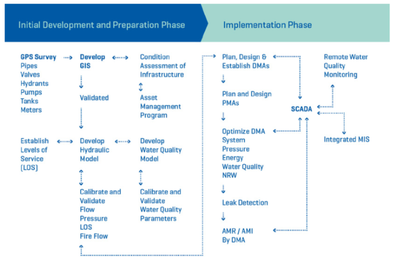
SWIT like GIS, Hydraulic Modeling, Asset Management should be developed in an initial preparation phase prior to implementing a capital intensive SWIT. Figure below shows a flow diagram of suggested preparation and implementation sequence of SWIT. (see IADB 2017, 41)

Method 1) CORRELATION AND REGRESSION

Correlation found in SWIT adoption

I look for some correlations between various key variables indicating adoption of certain SWIT solutions in the Brazil sample.

Assumptions

For simplicity, all variables have been recoded as binary 0/1
- 1 = (YES) includes {Yes, InConstruciton}
- 0 = (No) includes {No, DK}
Based on my understanding of the above, I divide the tools in 3 tiers of increasing complexity/innovation degree. Tier 1:
- LossMech = Q24_VolLossMech_Has
- GISpipes = Q58a_GIS_Pipe_Has
- HidrMod = Q60_HidrMod_Has Tier 2:
- DMA = Q62_DMA_Has,
- Press = Q65_PressSyst_Has,
- SCADA = Q68_SCADA_UtilLevel,
Tier 3:
- LeaksAn = Q39_LeaksDetection_Analyzed
- AMR = Q67b_MeterUtilLevel_AMR Yes = {Allmeters, SomeMeters, InConstr} NO = {Possible, Not USEd, }
- AMI = Q67c_MeterUtilLevel_AMI Yes = {Allmeters, SomeMeters, InConstr} NO = {Possible, Not USEd, }

Results correlation

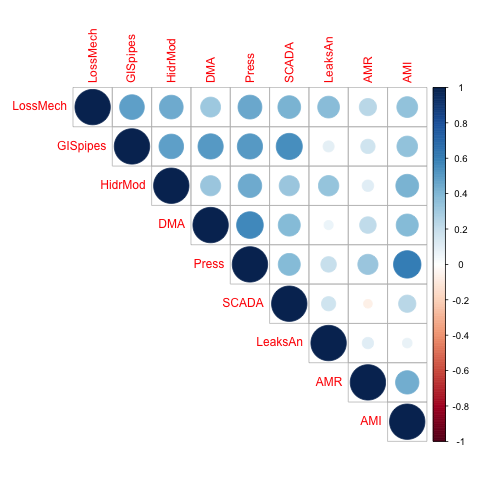
Based on a first check, the adoption of the SWIT technologies shows some expected results. Within tiers there is fairly strong correlation, but not a very noticeable pattern.

pacman::p_load(here, corrplot, ggcorrplot) 
load(here::here("output", "swit_sets.Rdata"))

# Building vectors of Variates and their own block corr matrix ----
X1 <- as.matrix(swit_sets[,3:5])   # the foundation SWITs ("LossMech" "GISpipes" "HidrMod")
# colnames(X1)
X2 <- as.matrix(swit_sets[,6:8])   # the foundation++ SWITs ("DMA"   "Press" "SCADA" )
# colnames(X2)
Y <- as.matrix(swit_sets[,9:11])  # the highest level meters ("LeaksAn" "AMR"     "AMI" )
# colnames(Y)

# Correlations Within VARIATES (vectors)  ------------------------------------------
X1_corr <- cor(X1) # fairly high positive corr 
X2_corr <- cor(X2)# fairly high positive corr 
Y_corr <- cor(Y)# fairly high positive corr  (except Leaks An)

All_corr <- cor(swit_sets[ ,3:11])
# All_corr

# corrplot(All_corr)

Results logistic regression

I use separate univariate multiple regressions on each of the binary dependent variables in Y (LeaksAn, AMR, AMI), which are considered the highest level of SWIT, to see if there is any effect of the lower tier SWITS. Nothing seems significant.

pacman::p_load(here, stargazer)

The downloaded binary packages are in /var/folders/0b/3s7cbr4d2kvft0fl2nkpqkdm0000gn/T//Rtmp8PzQeR/downloaded_packages

# Separate univariate multiple (LOGIT) regressions
LeaksAn.mod <- glm(LeaksAn  ~  LossMech + GISpipes + HidrMod + DMA + Press + SCADA, data=swit_sets, family = binomial(link="logit"))
# summary(LeaksAn.mod)

# # Marginal effects show the change in probability when the predictor or independent variable increases by one unit. 
# LeaksAn.mod.me <- logitmfx(LeaksAn  ~  LossMech + GISpipes + HidrMod + DMA + Press + SCADA, data=swit_sets)
 
AMR.mod <- glm( AMR  ~  LossMech + GISpipes + HidrMod + DMA + Press + SCADA, data=swit_sets, family = binomial(link="logit"))
#AMR.mod.me <- logitmfx( AMR  ~  LossMech + GISpipes + HidrMod + DMA + Press + SCADA, data=swit_sets)
 

 
AMI.mod <- glm( AMI ~  LossMech + GISpipes + HidrMod + DMA + Press + SCADA, data=swit_sets, family = binomial(link="logit"))
# summary(AMI.mod) 
#AMI.mod.me <- logitmfx( AMI ~  LossMech + GISpipes + HidrMod + DMA + Press + SCADA, data=swit_sets)
 

# 3 Y dep var individually studied
stargazer(LeaksAn.mod, AMR.mod ,AMI.mod, type = "html", digits=2,
             omit.table.layout = "#",
             star.cutoffs = c(0.05, 0.01, 0.001),
             #omit = "Constant",
             title="Univariate logistic regression models for SWIT most advanced tools")

**Univariate logistic regression models for SWIT most advanced tools**

	Dependent variable:

	LeaksAn	AMR	AMI

LossMech	2.14	1.41	0.55
	(1.37)	(1.29)	(1.53)

GISpipes	-1.57	0.40	-0.33
	(1.51)	(1.09)	(1.23)

HidrMod	1.62	-0.38	1.40
	(1.12)	(0.98)	(1.19)

DMA	-0.38	0.51	0.58
	(1.30)	(0.93)	(1.01)

Press	0.18	1.45	2.45^*
	(1.26)	(1.01)	(1.11)

SCADA	0.37	-1.88	-0.28
	(1.12)	(1.19)	(1.23)

Constant	-0.54	-0.88	-3.02^*
	(0.89)	(0.98)	(1.42)


Observations	39	39	39
Log Likelihood	-17.08	-22.84	-18.26
Akaike Inf. Crit.	48.15	59.68	50.52

Note:	p<0.05; p<0.01; p<0.001

# stargazer(LeaksAn.mod, AMR.mod ,AMI.mod, type="html", out="logit.htm")

Method 2) ASSOCIATION RULE MINING

This hypothesis can be explored borrowing from Association Rule Mining (a type of data mining analysis), which has applications in marketing, Market Basket Analysis, and many other industries with large datasets in which there can be association between objects of a set.

GOAL: identify association rules that fulfill a predetermined level of accuracy in the dataset

One method is the APRIORI algorithm (in R pckg arules::apriori()) to generate the most relevant set of rules from a given transaction data. It also shows the support, confidence and lift of those rules ( i.e., three measure that can be used to decide the relative strength of the rules)

Key Metrics

\[Support (item\ or\ itemsets)= \frac{Number\ of\ transactions\ with\ both\ A\ and\ B}{Total\ number\ of\ transactions} = P\left(A \cap B\right)\]

\[Confidence = \frac{Number\ of\ transactions\ with\ both\ A\ and\ B}{Total\ number\ of\ transactions\ with\ A} = \frac{P\left(A \cap B\right)}{P\left(A\right)}\]

\[Expected Confidence = \frac{Number\ of\ transactions\ with\ B}{Total\ number\ of\ transactions} = P\left(B\right)\]

\[Lift = \frac{Support {\left(A \cap B\right)}}{Support(A)*Support (B)} = \frac{P\left(A \cap B\right)}{P\left(A\right)*P\left(B\right)}\]

Hence \(Lift >1\) implies a positive relationship (higher than randomly selecting the two items combined)

Association rules found in SWIT adoption

I look at some key variables about adoption of certain SWIT solutions in the Brazil sample (all binary 0/1)

Assumptions

I only keep “Has GIS for Pipes,” although I have also 3 more variables about GIS (all give the same answer)
For simplicity in making the binary variables:
- 1 = (YES) includes {Yes, InConstruciton}
- 0 = (No) includes {No, DK}
Min supp = 0.01, minlen = 3, maxlen = 5, conf = 0.75 # set very high (Stronger rules)

Results

Based on the observations, the adoption of the SWIT technologies shows some expected results, and association patterns in adoption such as

{DMA, PressSyst , AMR} => {AMI}
{HidrModel, DMA , AMR} => {PressSyst}
{DMA, SCADA, AMR} => {GIS_Pipe}
etc.

although, when looking at the lift metric it is never higher than 1.7, which indicate weak association rules.

pacman::p_load(here, arules, arulesViz)

The downloaded binary packages are in /var/folders/0b/3s7cbr4d2kvft0fl2nkpqkdm0000gn/T//Rtmp8PzQeR/downloaded_packages

load(here::here("output", "swit_t.Rdata"))


# ----- FREQUENT ITEM-SETS with APRIORI
itemsetsAP <- apriori(swit_t,
  parameter = list(
    #target = "frequent itemsets",
    supp = 0.01, # itemset min support
    minlen = 3,
    maxlen = 7,
    conf = 0.75 # set very high (Stronger rules) 
  ),
  control = list(verbose = FALSE)
)
 
# interactive Graph-based VISUALIZATION
top20 <- head(itemsetsAP, n=20, by = "lift")
plot(top20, method = "graph",  engine = "htmlwidget")

i/n — PHASE I (Suppliers)

If the survey validates the prevailing lack of efficiency (high NWR), can we see any correlation with:

company features (ownership, size, state, urban/rural location, network lenght …)?
human resources (estimated by staff/served pop ratio) and technical capacity (technical staff/served pop ratio)?
systems in place to monitor (metering, leakage, illegality, customer complaints )?
degree of adoption of SWITS / smart technology?

Process

i/n — PHASE I (Suppliers)

As a proxy for reliability, the surveys asks about service interruptions in the past 12 months, the % of network affected and for how long (days). What are the main causes of service interruption?

(Main Reason 1 = maintenance) –> Connection with energy staff capacity?
(Main Reason 2 = energy) –> Connection with energy blackouts…?

Can we see any correlation with: + Degree of independence in governance? + Having (effective) CRM systems in place?

Process

i/n — PHASE I (Suppliers)

Certain suppliers involved in alleged corruption / changes of ownership occurred around survey + refer to Desk Research…

i/n — PHASE I (Suppliers) & PHASE 2 (Households)

Explore outcome affordability & (possibly) related variables to explore:
+ Financial assets + Relevant tariff scheme + Financial efficiency tools + Governance structure

Process

i/n — PHASE I (Suppliers) & PHASE 2 (Households)

(In combination PHASE I & PHASE II) could explore outcome affordability & (possibly) related variables to explore:
- Financial assets
  - Relevant tariff scheme
- Financial efficiency tools
- Governance structure

Process

i/n — PHASE I (Suppliers) & PHASE 2 (Households)

(In combination PHASE I & PHASE II) could explore outcome quality & (possibly) related variables to explore:
- …
- …
- …

Process

IADB. 2017. “Evaluation of Smart-Water-Infrastructure-Technologies-(SWIT).”

Analysis of Survey WSS Operators Brazil

Last run: April 21, 2022

1/n — PHASE I (Suppliers)

Method 1) CORRELATION AND REGRESSION

Correlation found in SWIT adoption

Assumptions

Results correlation

Results logistic regression

Method 2) ASSOCIATION RULE MINING

Key Metrics

Association rules found in SWIT adoption

Assumptions

Results

i/n — PHASE I (Suppliers)

Process

i/n — PHASE I (Suppliers)

Process

i/n — PHASE I (Suppliers)

i/n — PHASE I (Suppliers) & PHASE 2 (Households)

Process

i/n — PHASE I (Suppliers) & PHASE 2 (Households)

Process

i/n — PHASE I (Suppliers) & PHASE 2 (Households)

Process