Descriptive Statistics of Survey WSS Operators Brazil
Last run: April 21, 2022
Exploratory Data Analysis of WSS Operators Sample in Brazil
The observation of survey outcomes will compare across potential relevant features:
- Ownership/type and
- Size of covered area
- Service mix (W/S/W+S)
- (possibly) Prevalence of urban vs rural coverage vs
- (Age)
- (State)
Here is a very basic distribution of our sampled Suppliers in Brazil, by STATE (UF), Ownership Type and size of Coverage reach
load(here::here("output", "tbl_uf_own_cov.Rdata"))
# class(tbl_uf_own_cov)
caption <- "Sampled Suppliers in Brazil, by STATE (UF), Ownership Type and size of Coverage reach"
covtable <- pandoc.table.return(tbl_uf_own_cov,
                                          keep.line.breaks = F,
                                          style = "multiline",
                                          justify = "lcrr",
                                          caption = caption
                                          )

cat(covtable)| NM_ESTADO | Q1_ownership_lbl | Cov_pop_rango_lbl | n |
|---|---|---|---|
| ACRE | Public | Large 500k-1m | 1 |
| ALAGOAS | Other | Large 1m-10m | 1 |
| AMAPÁ | Other | Large 500k-1m | 1 |
| AMAZONAS | Public | Medium 50-100k | 1 |
| AMAZONAS | Other | Medium 300-500k | 1 |
| BAHIA | Other | Mega >10m | 1 |
| CEARÁ | Other | Large 1m-10m | 1 |
| DISTRITO FEDERAL | Other | Large 1m-10m | 1 |
| ESPÍRITO SANTO | Other | Large 1m-10m | 1 |
| GOIÁS | Public | Small 10-50k | 1 |
| MARANHÃO | Other | Large 1m-10m | 1 |
| MATO GROSSO | Public | Very Small <10k | 1 |
| MATO GROSSO | Public | Medium 200-300k | 1 |
| MINAS GERAIS | Public | Small 10-50k | 1 |
| MINAS GERAIS | Other | Mega >10m | 1 |
| PARÁ | Public | Large 1m-10m | 1 |
| PARAÍBA | Other | Large 1m-10m | 1 |
| PARANÁ | Other | Mega >10m | 1 |
| PERNAMBUCO | Other | Large 1m-10m | 1 |
| RIO DE JANEIRO | Public | Medium 300-500k | 1 |
| RIO DE JANEIRO | Other | Mega >10m | 1 |
| RIO GRANDE DO NORTE | Other | Large 1m-10m | 1 |
| RIO GRANDE DO SUL | Public | Medium 50-100k | 1 |
| RIO GRANDE DO SUL | Public | Large 1m-10m | 1 |
| RIO GRANDE DO SUL | Private | Medium 50-100k | 1 |
| RIO GRANDE DO SUL | Other | Large 1m-10m | 1 |
| RONDÔNIA | Public | Large 1m-10m | 1 |
| SANTA CATARINA | Public | Small 10-50k | 1 |
| SANTA CATARINA | Public | Medium 50-100k | 1 |
| SANTA CATARINA | Public | Large 500k-1m | 1 |
| SANTA CATARINA | Private | Large 1m-10m | 1 |
| SÃO PAULO | Public | Very Small <10k | 1 |
| SÃO PAULO | Public | Small 10-50k | 1 |
| SÃO PAULO | Public | Medium 200-300k | 1 |
| SÃO PAULO | Public | Mega >10m | 1 |
| SÃO PAULO | Private | Large 1m-10m | 2 |
| SÃO PAULO | Other | Mega >10m | 1 |
| SERGIPE | Other | Large 1m-10m | 1 |
| Total | - | - | 39 |
Legislative Context
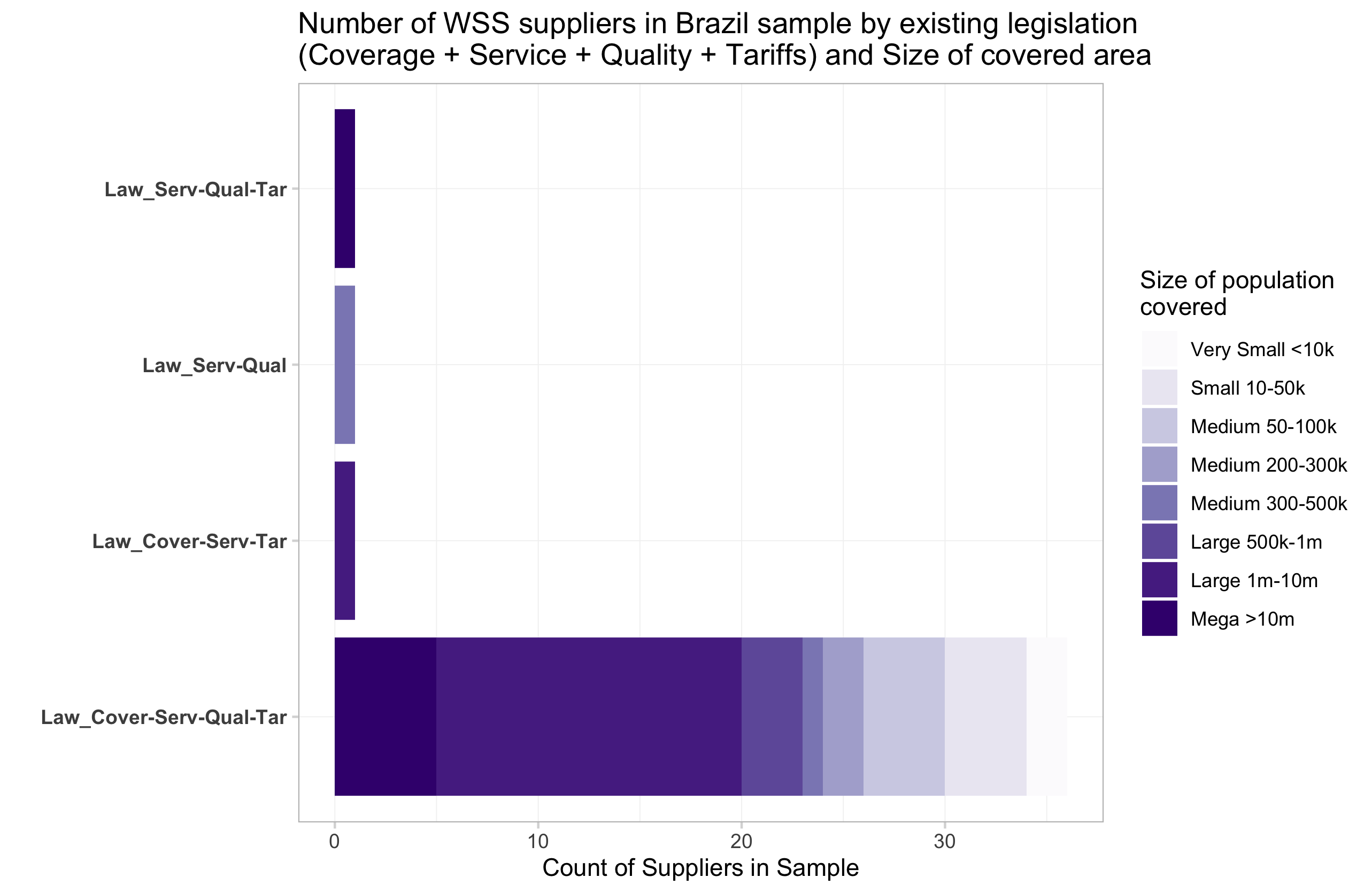
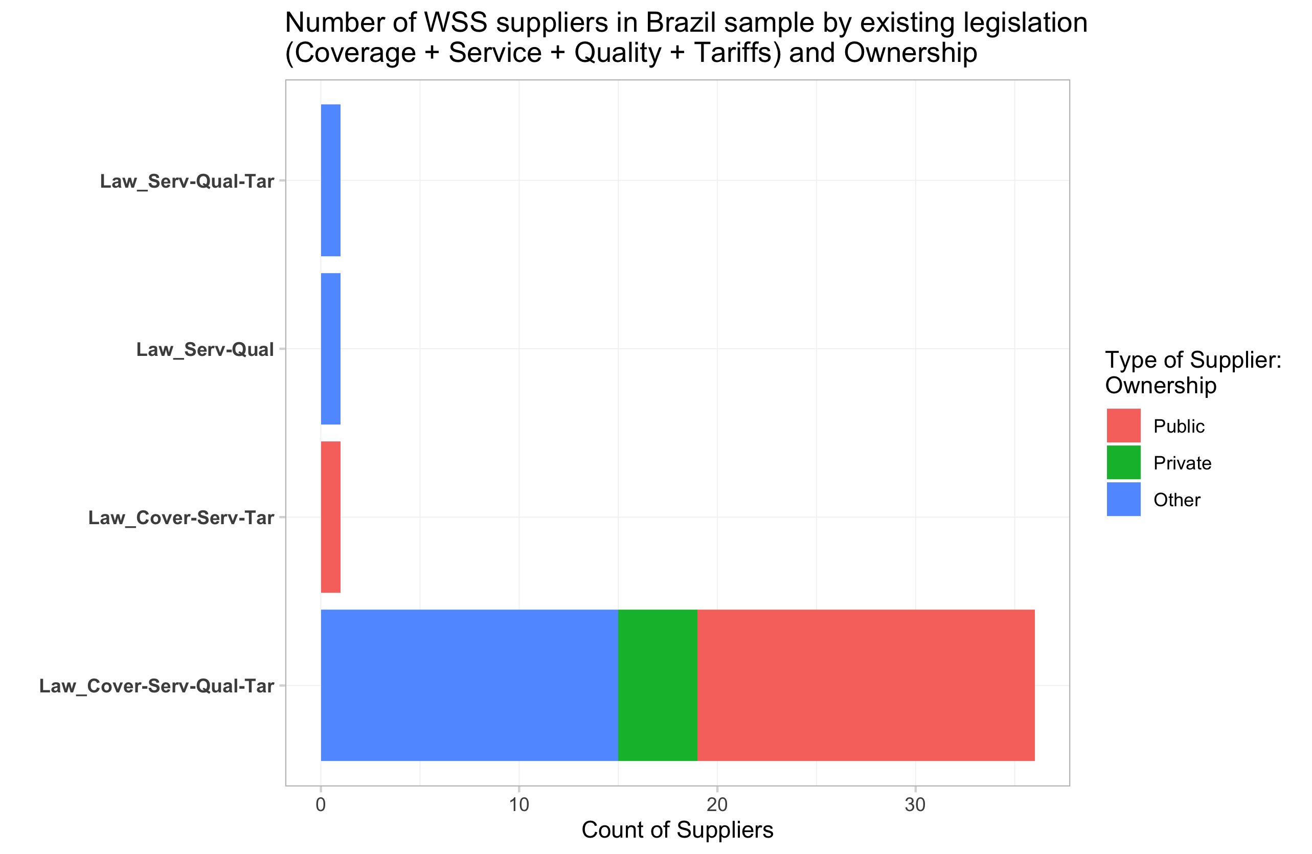
- Overall, the majority of the Suppliers declare they operate in a context where there is legislation for key operational aspects such as:
- Coverage Areas
- Service
- Quality
- Tariffs
1) COVERAGE & SERVICE
Summary of key coverage numeric variable
load(here::here("output", "tbl_descstat_cov.Rdata"))
# class(tbl_descstat_cov)

caption <- "Summary of Coverage variables"
var.summary <- pandoc.table.return(tbl_descstat_cov ,
                                              keep.line.breaks = TRUE,
                                              round = 2,
                                              big.mark = ",",
                                              justify = "llrrrrrr", # OKKIO AL # DI COLONNE
                                              caption = caption, style = "multiline",
                                              split.table = Inf
                                              )

cat(var.summary)| Variable | unit_of_analysis | N | Mean | Std. Dev. | Median | Min | Max |
|---|---|---|---|---|---|---|---|
| N_cov_states | NA | 39 | 1.79 | 2.47 | 1 | 1 | 12 |
| N_cov_mun | Num of Municipio covered (Annex) | 39 | 88.44 | 140.6 | 22 | 1 | 629 |
| Q2_CovMun_decl | Num of Municipio covered (Respondent) | 39 | 88.46 | 140.6 | 22 | 1 | 629 |
| totpop2018 | Tot Pop in covered Mun (IBGE2018) | 39 | 4,530,220 | 6,759,477 | 1,707,440 | 3,928 | 29,879,718 |
| Q44_Past12m_Interr_RespTime | NA | 31 | 1.79 | 3.41 | 1 | 0.04 | 18.91 |
| Q5a_Urb_Perc2 | NA | 19 | 83.92 | 14.87 | 90 | 52 | 99 |
Area(s) covered vs. service
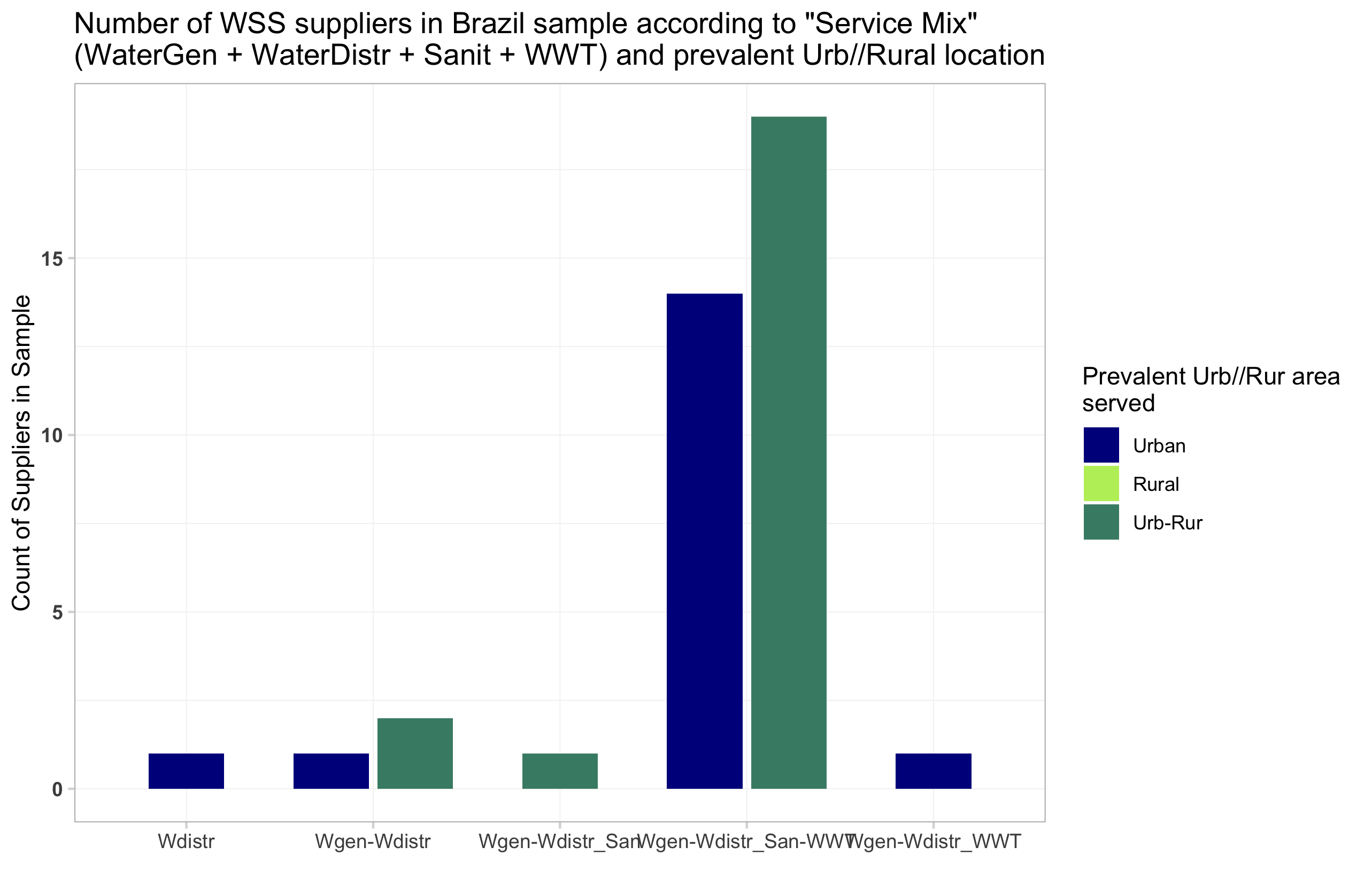
Is there any difference between the Product MIX
Q9a_d_Mix_combvs the URB-RUR MIX of the supplierQ4_UrbRur_Mix1?
There are no suppliers serving exclusively rural area. No remarkable differences in the Product MIX across the URB / RUR MIX types
NEXT:… (?) Is the urbanization process (size, local distribution, rate) causing the lack (access, quality, affordability ) to service in the region (controlling for physical assets / hydrological condition, pop #, etc) ? ??
Summary of key service charateristics
the WSS suppliers in the sample as of April 21, 2022, …
load(here::here("output", "tbl_descstat_covserv.Rdata"))
# class(tbl_descstat_cov)

caption <- "Summary of Service variables"
var.summary <- pandoc.table.return(tbl_descstat_covserv ,
                                              keep.line.breaks = TRUE,
                                              round = 2,
                                              big.mark = ",",
                                              justify = "llrrrrrr", # OKKIO AL # DI COLONNE
                                              caption = caption, style = "multiline",
                                              split.table = Inf
                                              )

cat(var.summary)| Variable | unit_of_analysis | N | Mean | Std. Dev. | Median | Min | Max |
|---|---|---|---|---|---|---|---|
| Q7a_Volume_Res_Perc | % of m3 | 38 | 87.27 | 7.22 | 89 | 60 | 95.92 |
| Q7b_Volume_Com_Perc | % of m3 | 37 | 7.91 | 4.26 | 7.5 | 0.13 | 20 |
| Q7c_Volume_Ind_Perc | % of m3 | 37 | 1.89 | 2.9 | 0.7 | 0 | 13.3 |
| Q7d_Volume_Inst_Perc | % of m3 | 37 | 3.14 | 2.89 | 2.05 | 0 | 13.3 |
| Q10a_Wconn_Res | Num connections water | 38 | 799,607 | 1,388,985 | 215,680 | 1,040 | 7,172,000 |
| Q10b_Wconn_Tot | Num connections water | 39 | 1,008,353 | 1,738,252 | 314,182 | 1,485 | 9,053,000 |
| Q10c_Wconn_Act | Num connections water | 39 | 888,812 | 1,549,006 | 295,460 | 1,190 | 7,987,000 |
| Q11a_Sconn_Res | Num connections sanitation | 32 | 444,860 | 1,104,293 | 79,099 | 2,097 | 5,984,000 |
| Q11b_Sconn_Tot | Num connections sanitation | 35 | 597,450 | 1,362,863 | 106,000 | 2,275 | 7,495,000 |
| Q11c_Sconn_Act | Num connections sanitation | 34 | 568,008 | 1,256,892 | 118,875 | 2,198 | 6,718,000 |
| Q12a_m3_In_Res | m3 water entering system | 20 | 127,187,676 | 213,537,966 | 38,813,618 | 467,500 | 833,099,200 |
| Q12b_m3_In_Tot | m3 water entering system | 39 | 210,130,900 | 3.37e+08 | 61,092,028 | 190,600 | 1.631e+09 |
| Q13_m3_Fatt_Tot | m3 water billed | 39 | 1.18e+08 | 182,513,737 | 24,591,156 | 123,600 | 785,720,000 |
| Q13a_m3_Fatt_Res_Perc | % of m3 water billed | 38 | 85.31 | 9.31 | 87.33 | 52 | 95.23 |
| Q13b_ReaisFatt_Tot | Revenue in Reais | 38 | 746,668,127 | 1.177e+09 | 214,512,932 | 546,573 | 4.601e+09 |
| Q13c_ReaisFatt_Res_Perc | % Residential of revenue in Reais | 38 | 79.07 | 9.4 | 78.38 | 56.46 | 95 |
| NRWm3_pct | % of m3 Water (in the system) NOT billed | 39 | 38.84 | 16.13 | 37.38 | 6.38 | 69.66 |
| Q23_Network_km | km | 39 | 80,829 | 308,791 | 4,158 | 9 | 1,828,660 |
| Q27_IndivMeter_Perc | % of connections | 38 | 86.3 | 24.1 | 99 | 12 | 100 |
| Q40_NetworkYrlyInspected_Perc | % of network | 22 | 70.73 | 37.13 | 89.5 | 2.3 | 100 |
| Q43_Past12m_Interr_PercAff | % | 25 | 38.51 | 34.48 | 30 | 0 | 100 |
NRW % levels
Lit Input: Some key determinants of high NRW are: 1. The cost of implementing counter-measures 2. A political cost associated with the control of unauthorized consumption in marginalized ares 3. A cost to those people who benefit from corruption 4. Technical cost of shortening leakage detection time & improving pressure management (especially when the cost of pumping more raw water is 0 or low) [see González-Gómez, García-Rubio, and Guardiola (2011), pp. 33-35; ch. 1].
Based on the information collected via the survey, we can estimate NRW as per International Water Association’s (IWA) definition: NRW is defined as water that is placed into a water distribution system that is not billed to customers. Our derived indicator is NRWm3_pct { = (Q12b_m3_In_Tot - Q13_m3_Fatt_Tot) / Q12b_m3_In_Tot *100 }
load(here::here("output", "BRA_NRW.Rdata"))

# class(tbl_descstat_cov)

# SIMPLE TABLE WITH FILTER
BRA_NRW %>% dplyr::select(-M1_oper_id, -Q12b_m3_In_Tot, -Q13_m3_Fatt_Tot) %>%
    dplyr::arrange(NM_ESTADO) %>%
    DT::datatable(.,
                  elementId = NULL,
                 # filter = 'top',  # Problem if there are empty cells !!!
                  extensions = 'Buttons',
                  options = list( pageLength = 50,searchHighlight = TRUE,   dom = 'Bfrtip', buttons = c( 'csv', 'excel','pdf'))
    ) %>%
    # helper functions
        DT::formatRound('NRWm3_pct', 1) %>%
        DT::formatStyle( 'NRWm3_pct', backgroundColor =  'yellow') %>%
        DT::formatStyle( 'NRWm3_pct', color = styleInterval( 50, c('black', 'red')) )
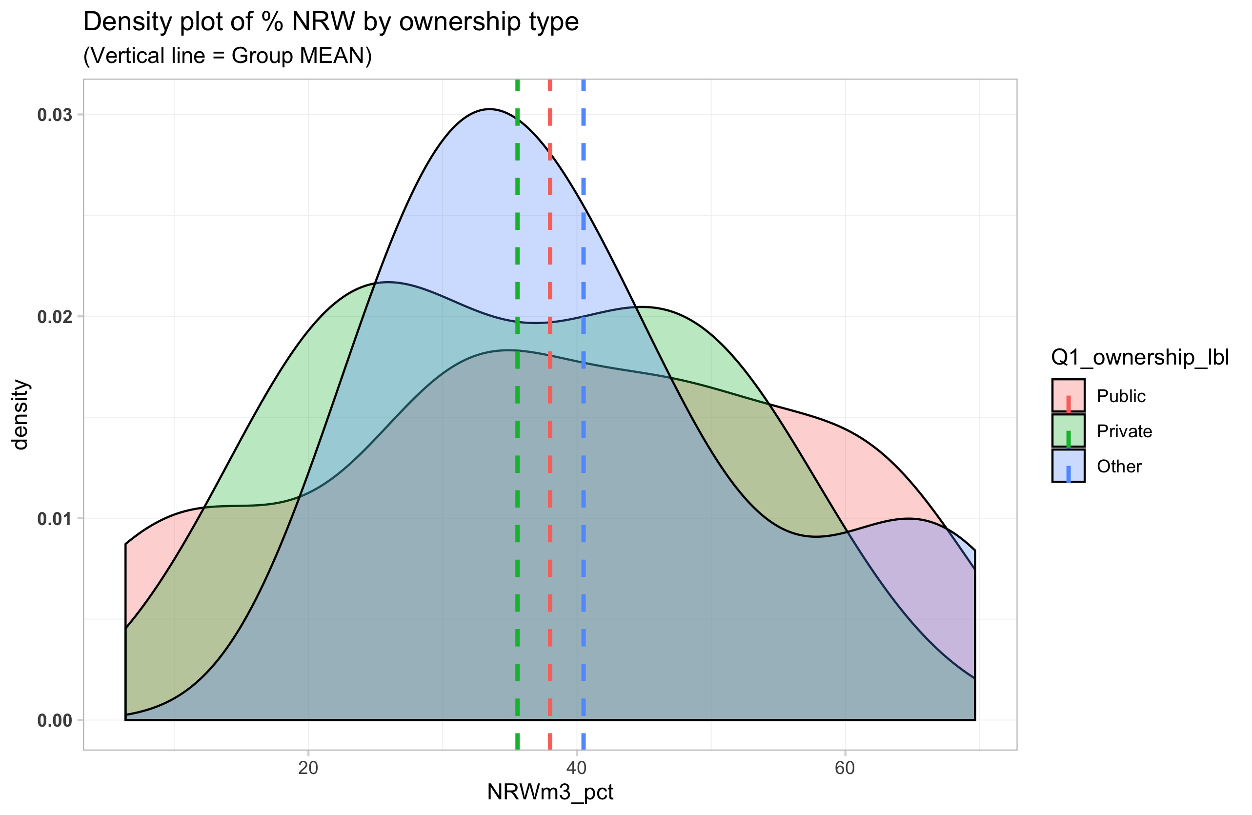
Initial exploration shows that:
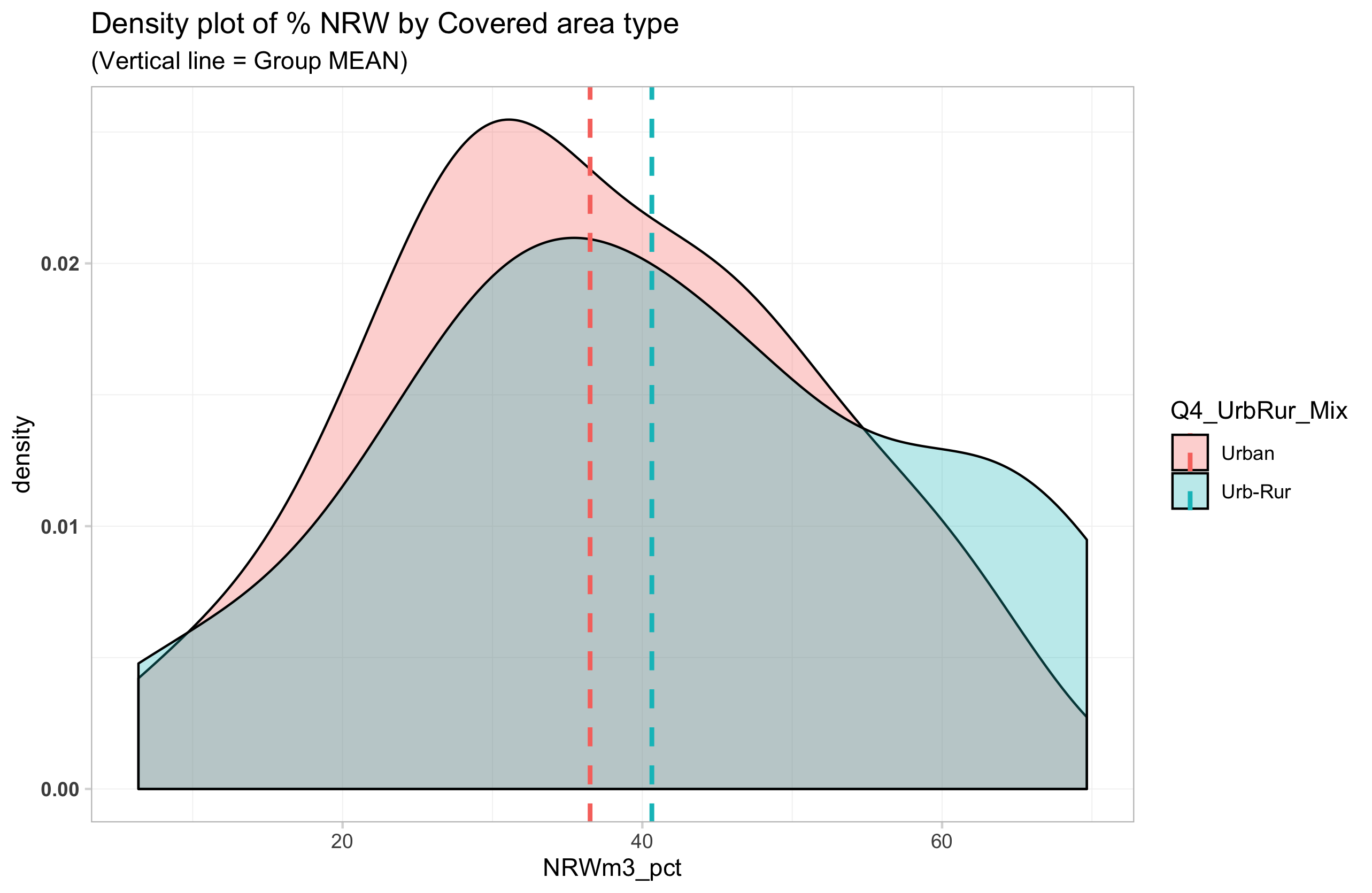
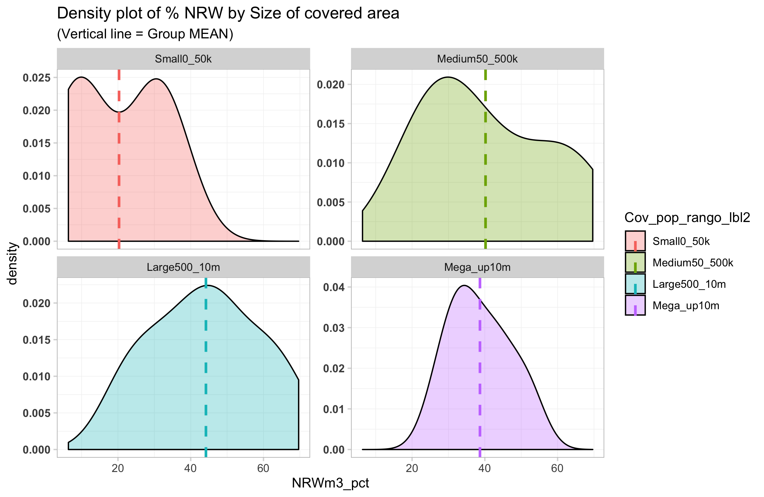
- On average, the % NWR varies quite dramatically across different ownership types (PUBLIC-owned 32% < Other 38% < Private 60% (more dispersed))
- Mean % NWR is lower for suppliers exclusively serving urban areas (34%) than for suppliers servin mixed-urb-rur (43%) … but sems quite disperserd.
- On average, the size of served population, is also a great source of variation in the %NRW - highest found in 500-900k size (58%) and smallest in 10-50k size (7%)
NRW correlation with “suspected” determinant factors
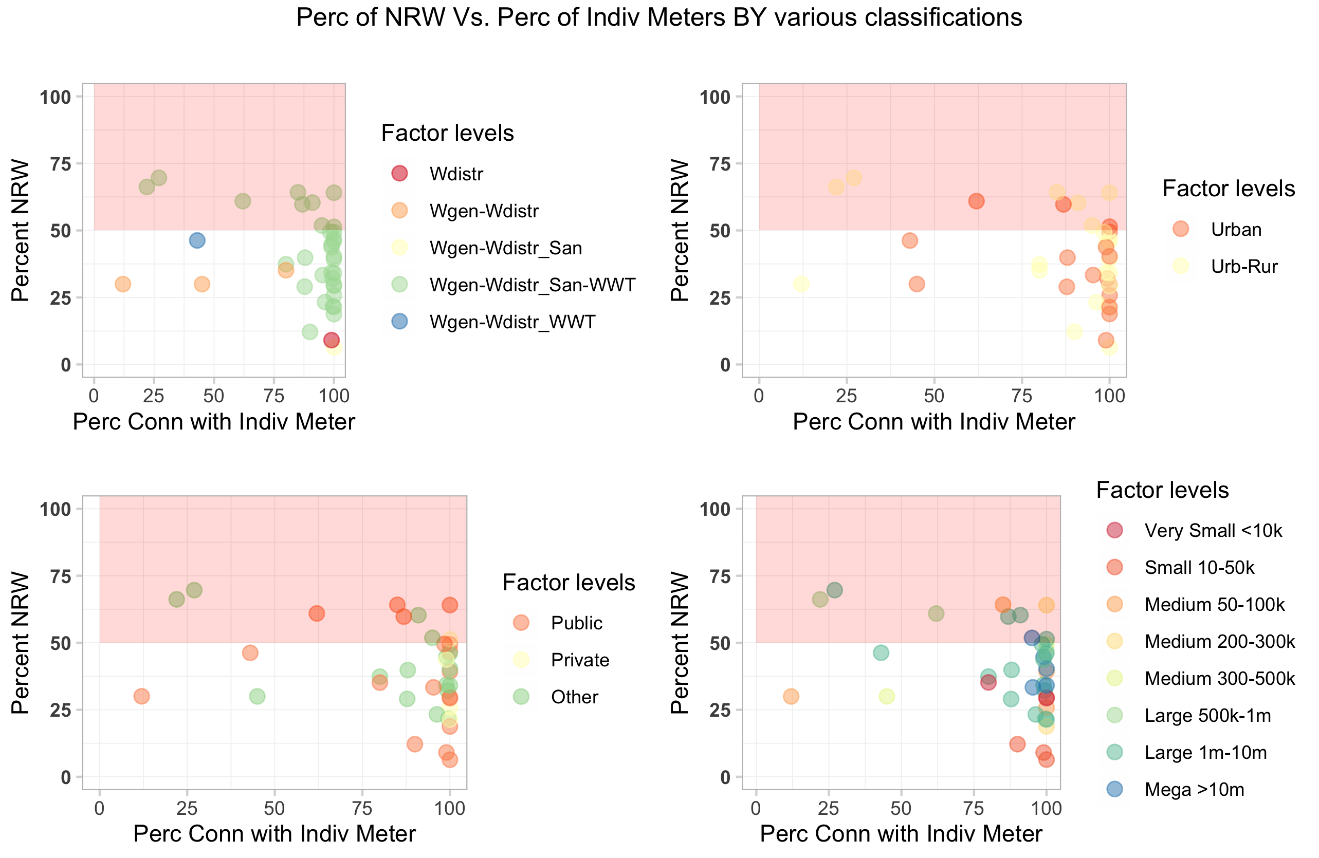
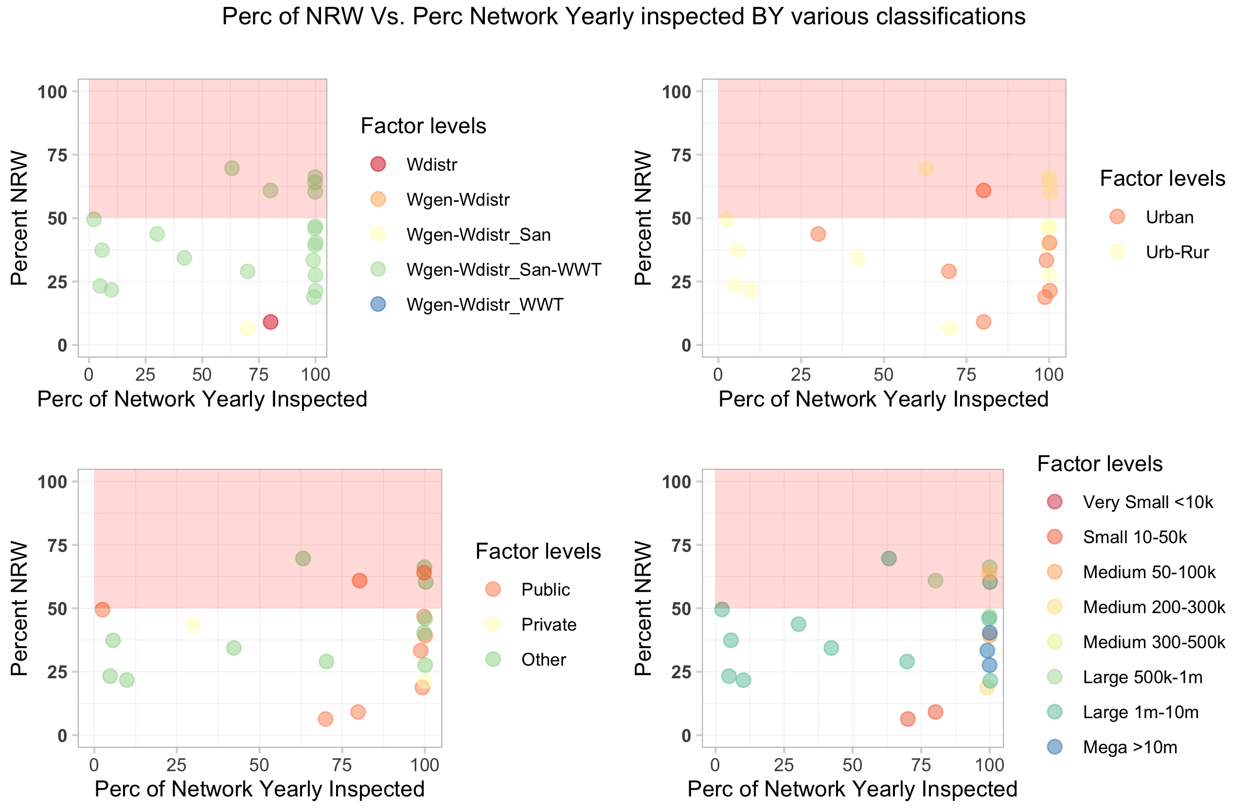
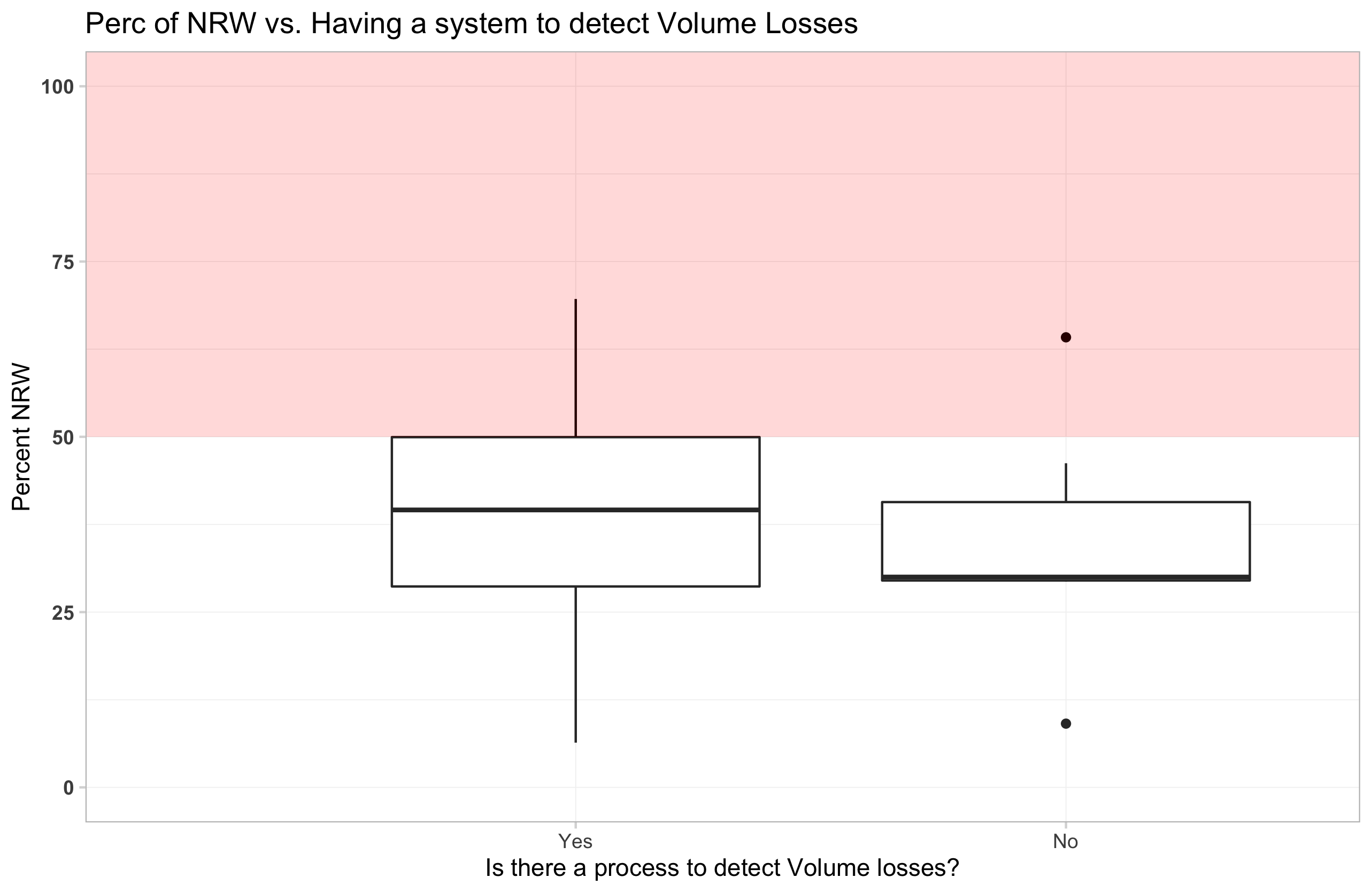
Visually explore whether the % of NRW shows any type of correlation with some variables that could be relevant:
Q27_IndivMeter_Perc–> no stryking connection
Q40_NetworkYrlyInspected_Perc–> no stryking connection
Q24_VolLossMech_Has–> most suppliers say “Yes” (have a system to record VOLUME LOSSES)
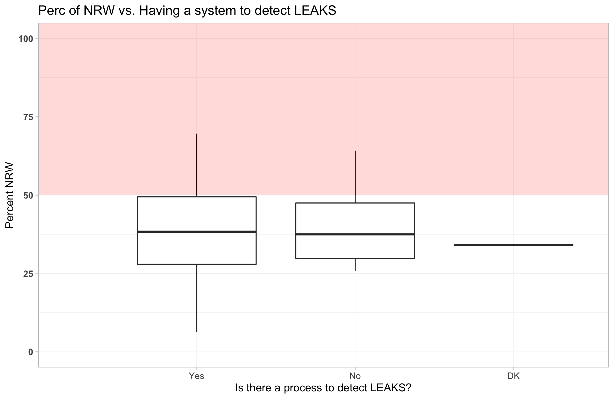
Q39_LeaksDetection_Analyzed–> most suppliers say “Yes” (have a systematic campaign to detect ruptures and LEAKS) and those cases show a somewhat lower NRW
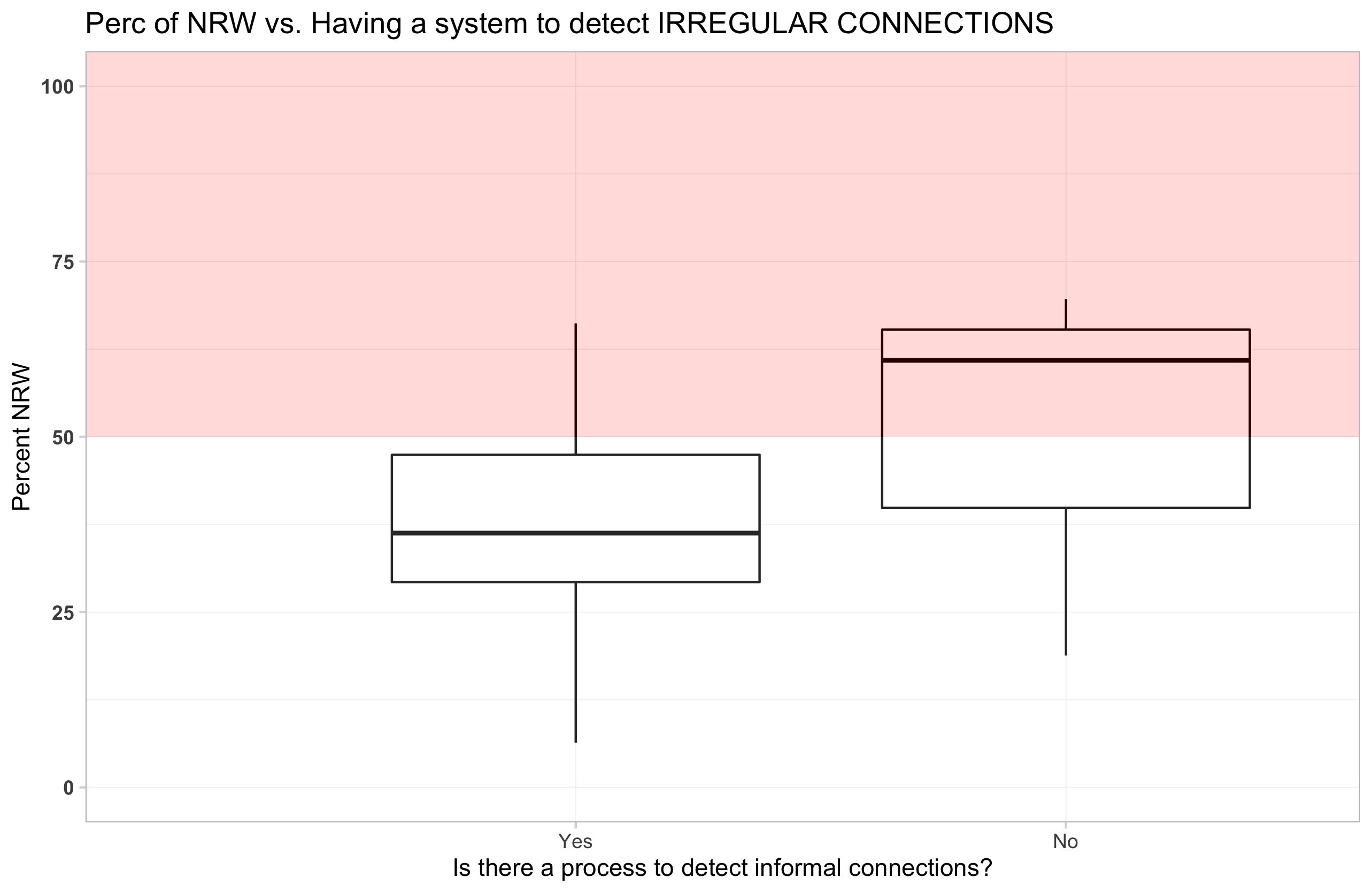
Q41_ClandConn_Analyzed–> the vast majority suppliers say “Yes” (have a system) and those cases show a significantly lower NRW (for now the NO sub-sample is too small to further analyze)
NEXT … Further exploration ….. + Exist procedim for estimation of vol loss/ (Q24)
* (?) Is the year of operation anywhere connected with efficiency?
* (?) Is thestack of laws connected with efficiency (Expected inverse relation)??Q8a_c_Leg_combQ8a_LegInst_CoverQ8b_LegInst_DirServ“Q8c_LegInst_DirQualQ8d_LegInst_Tarif,”
Reliability of the service (Interruptions)
Lit Input: Performance can improve with: 1) carefully designed private sector participation in service provision 2) regulatory agencies that are transparent, accountable, and free of political interference, 3) strong accountability mechanisms for SOE. (see Andrés, Schwartz, and Guasch 2013 ).
Y + Reliability = Q4… Q45 interruptions X + location + size + age? Q6 + Quality regulation (q8c) + SWIT penetration ? + % eng in staff + % IT in staff?
The table below shows responses related to the incidence of service interruptions in the past 12 months.
load(here::here("output", "BRA_REL.Rdata"))

# class(tbl_descstat_cov)

# SIMPLE TABLE WITH FILTER
#datatable(data= BRA_REL  , filter = 'top')
DT::datatable(BRA_REL,
                  elementId = NULL,
                  #filter = 'top',
                  extensions = 'Buttons',
                  options = list( pageLength = 50,  dom = 'Bfrtip', buttons = c( 'csv', 'excel')),
                  caption = 'Individual Supplier\'s Responses about Service Interruptions'
) %>%
    formatRound("Perc of network affected", 1) %>%
    formatRound("Avg # days of interruption", 1) %>%
        DT::formatStyle("Perc of network affected", color = styleInterval( 50, c('black', 'red')) )
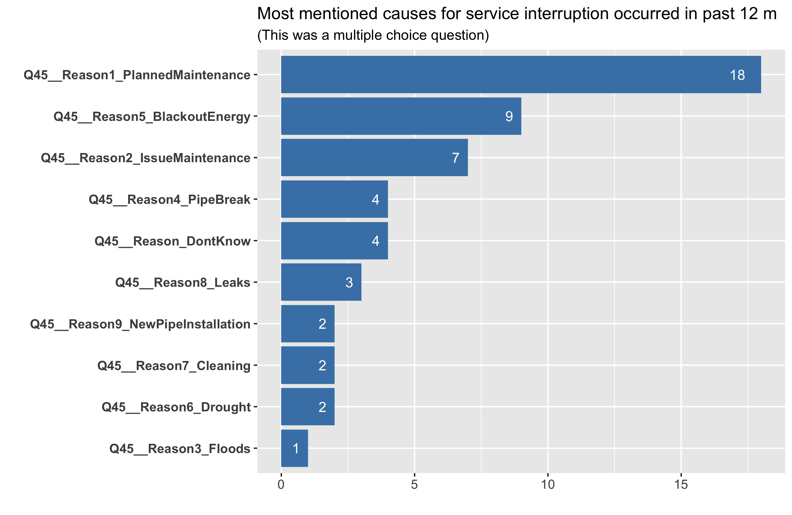
The chart below shows the most frequent causes for service interruption p
2) SWIT
Use of SWIT still not widespread for various barriers: + high capital investments + slow cost recovery + limited technical capacity, particularly for small utilities, + lack of integration between different technologies
Summary of SWIT adoption in the Brazil sample
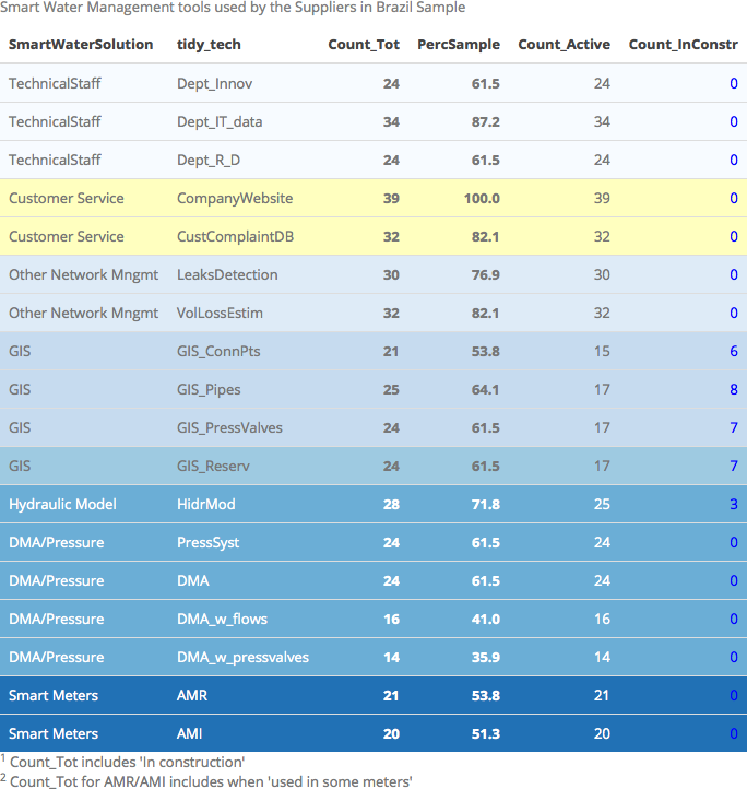
The table belows shows to what degree the WSS suppliers in the sample nrow(BRA_REL) already adopt various types of Smart Water Management: dedicated R&D and IT departments, Network Management systems, GIS, Hidraulic Models, DMA & pressure management, and Smart meters.
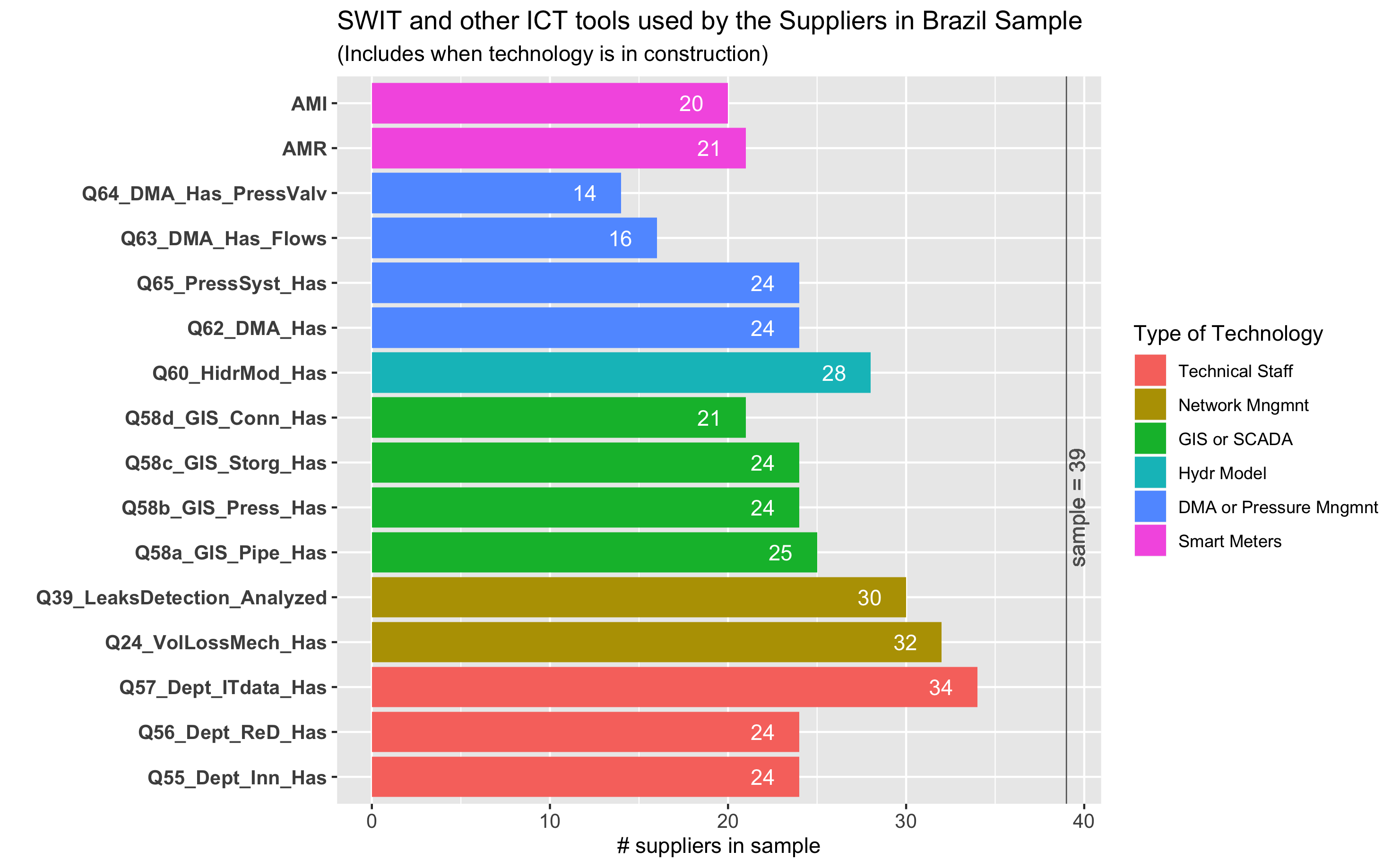
The % of adoption (albeit Count includes when tools are still “in construction”) appear quite high.
NOTES + Some of the respondents are actually large companies comglomerate, so will have to understand better their distribution by size and ownership…. + Even when companies say “yes” to the adoption (e.g. smart meter) it may be just a pilot…
Below is a different graph to show the degree of adoption of various types of technologies.
3) CORPORATE GOVERNANCE
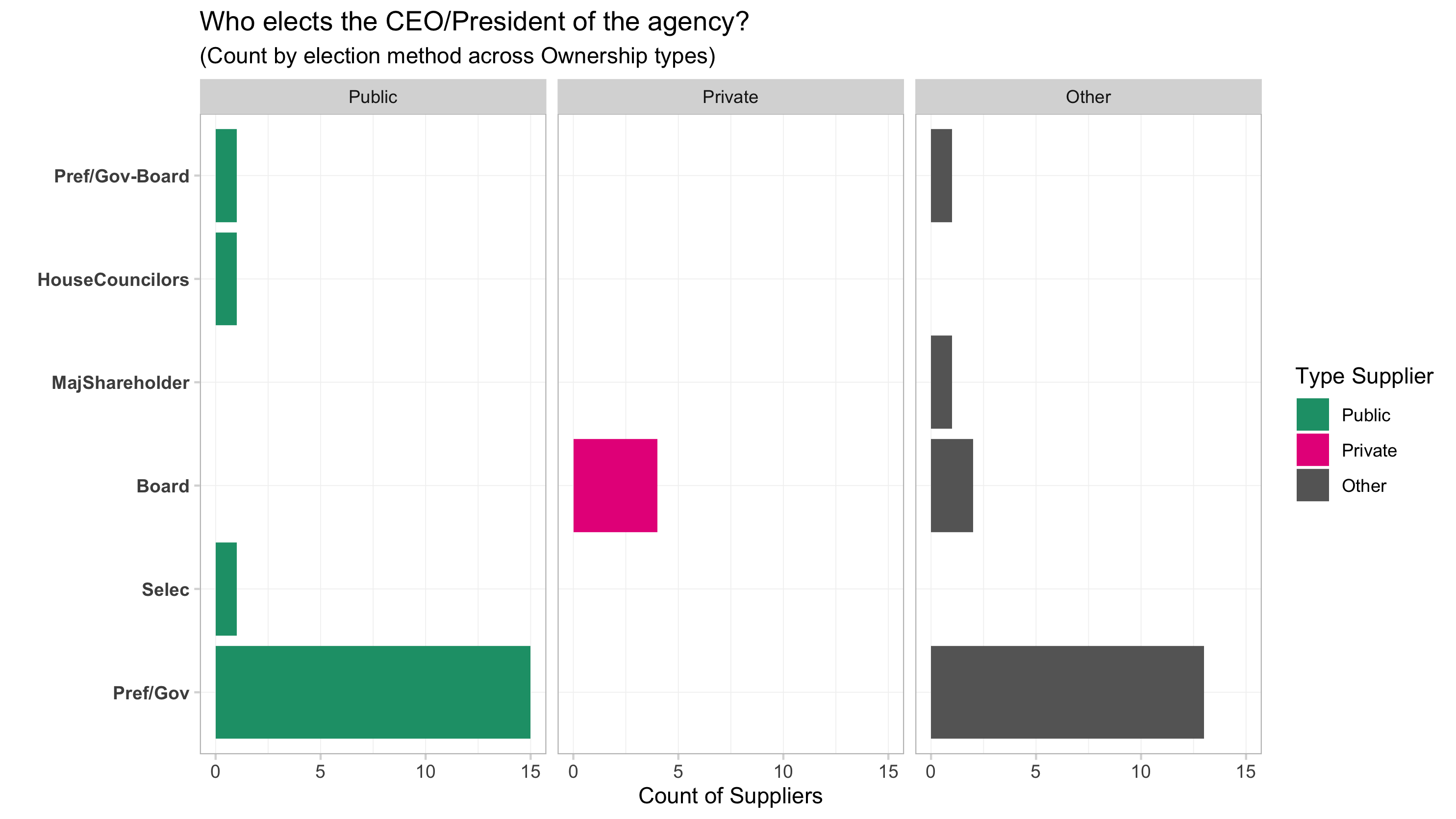
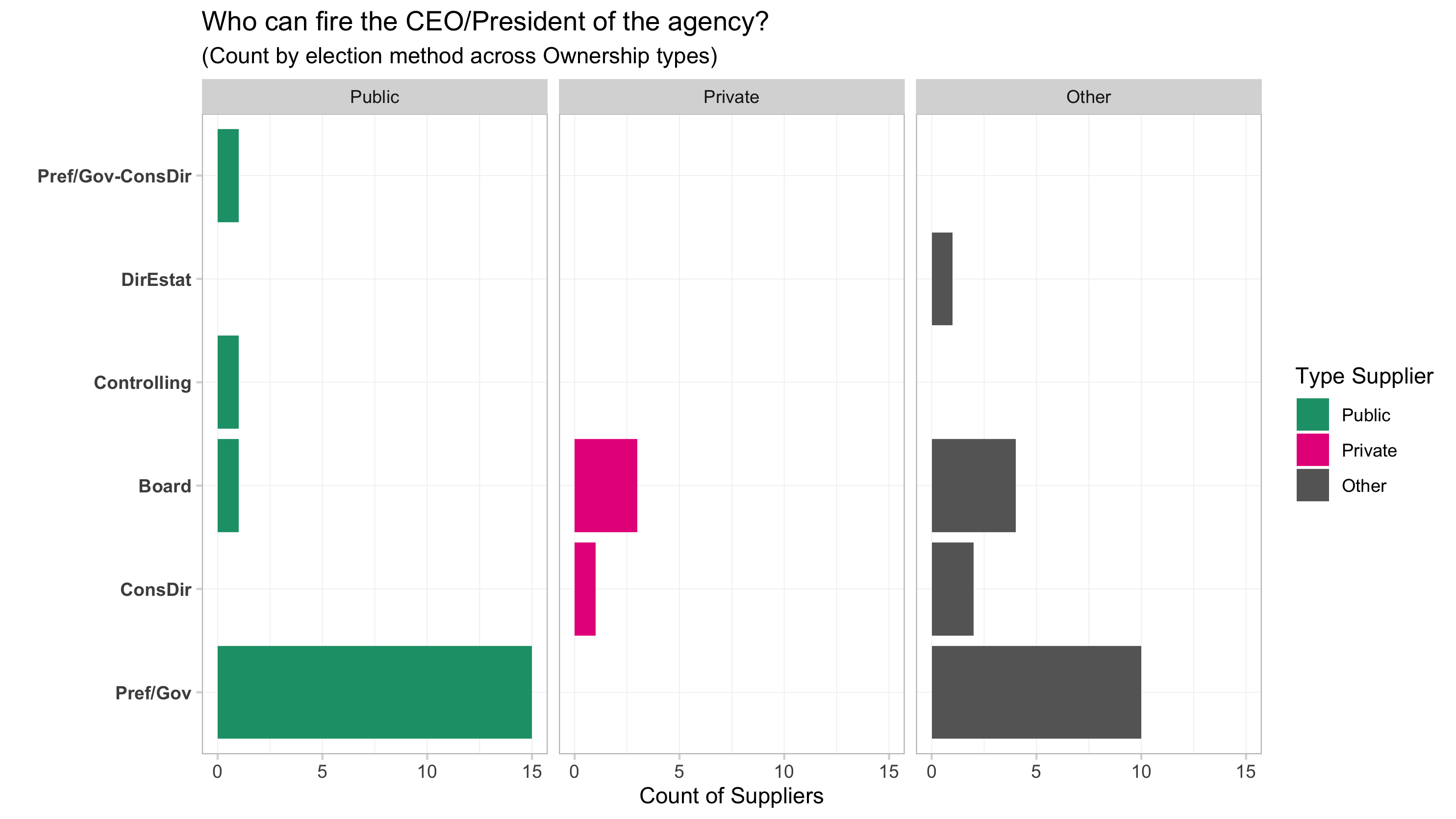
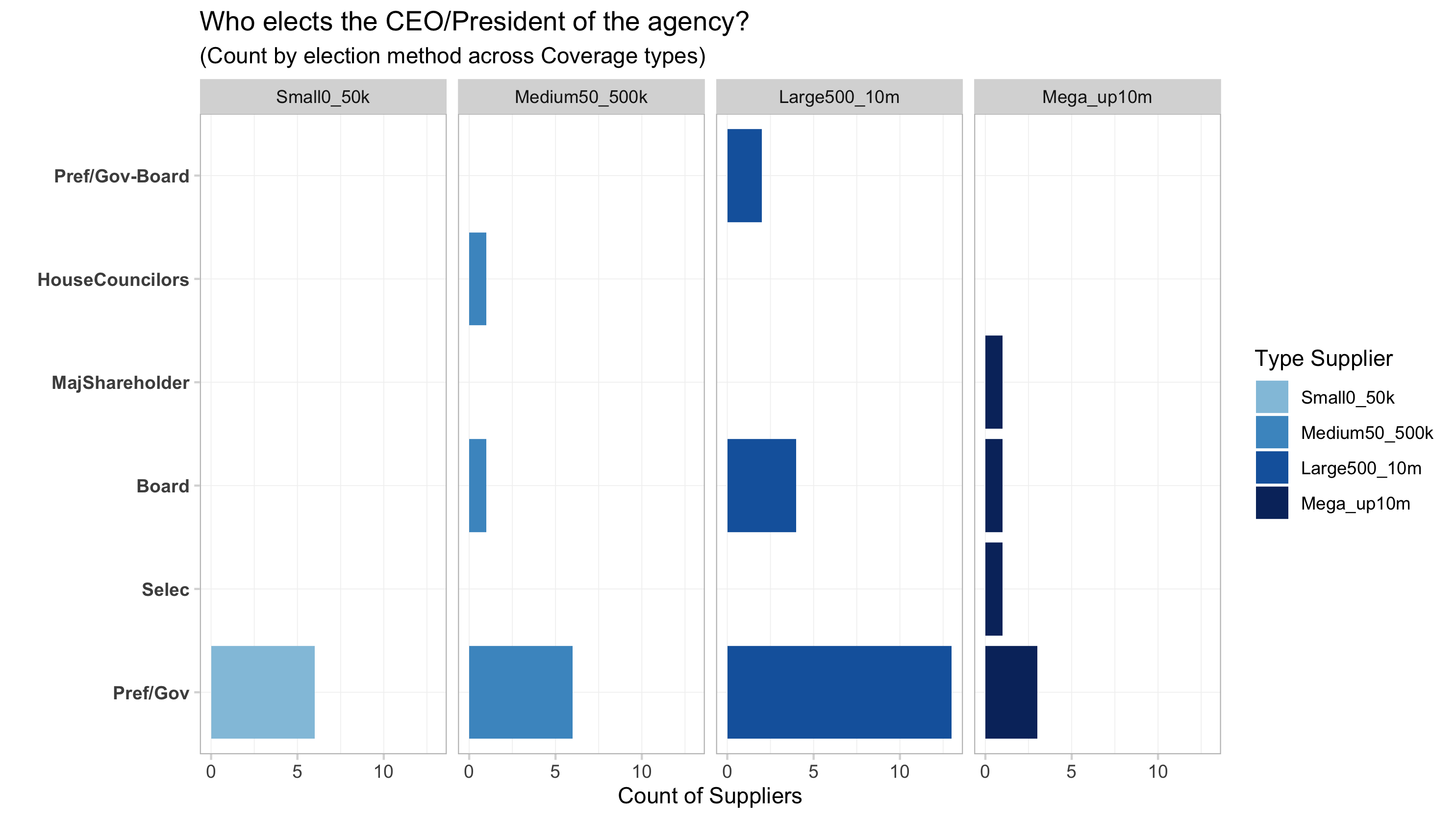
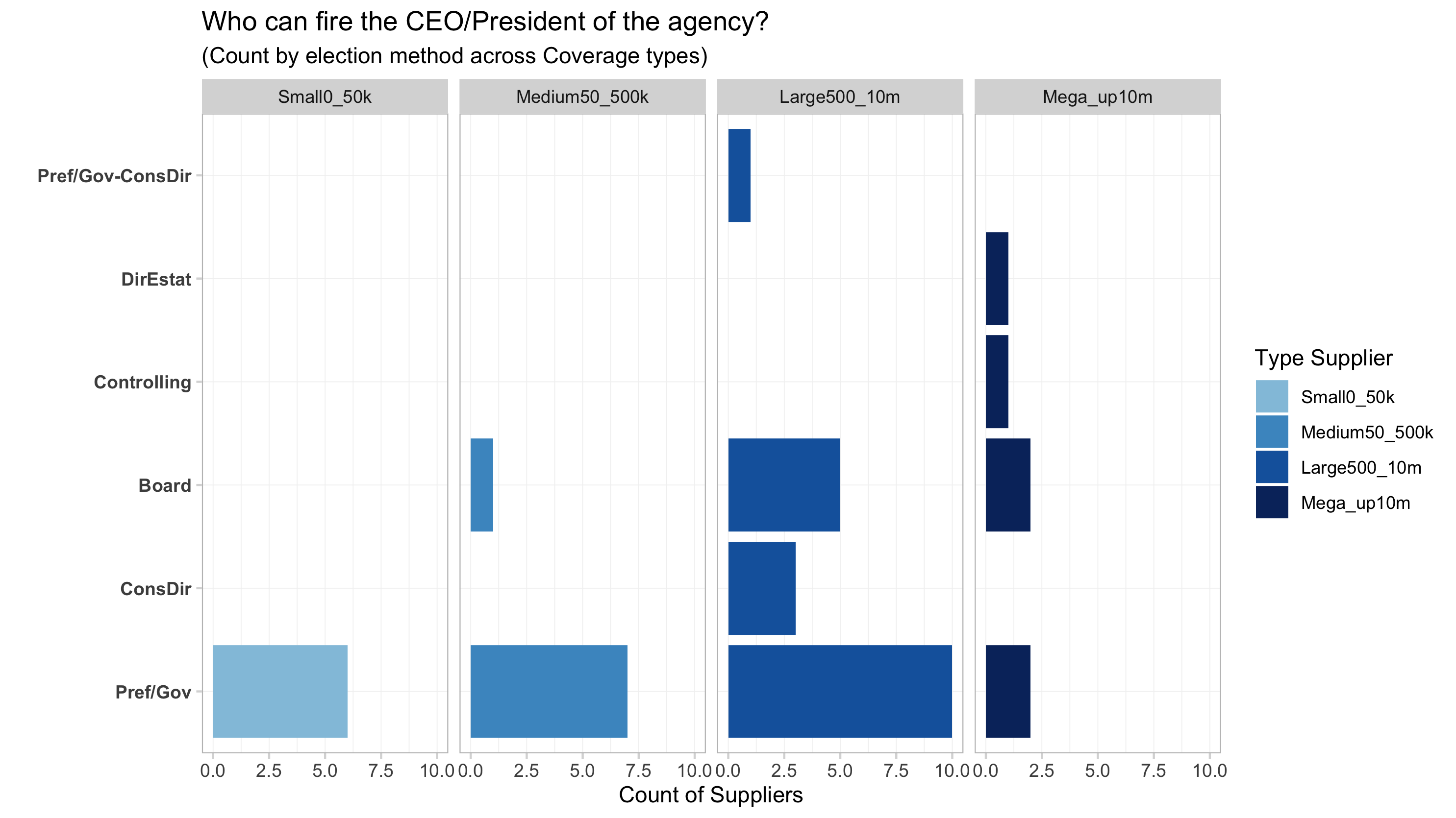
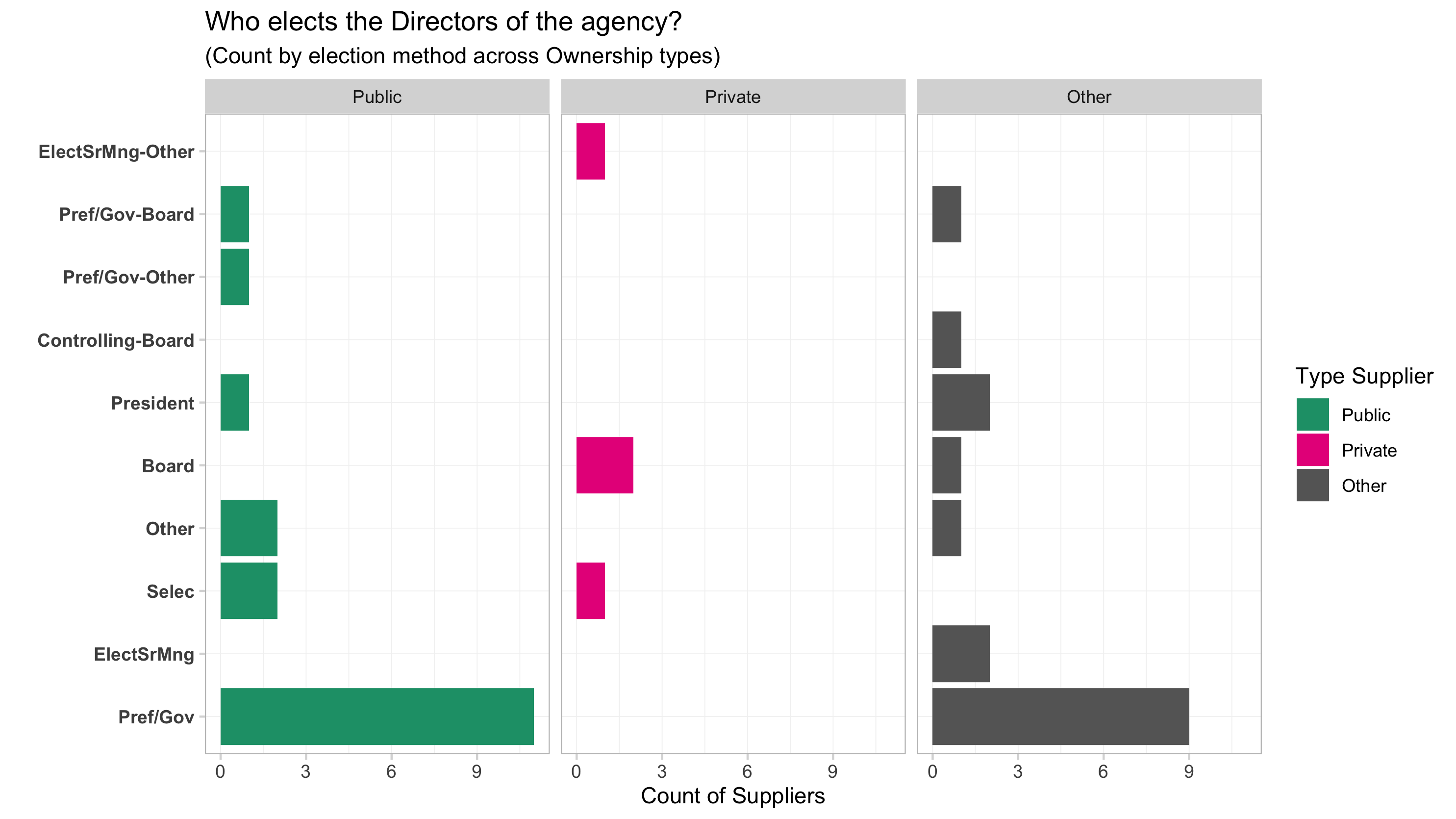
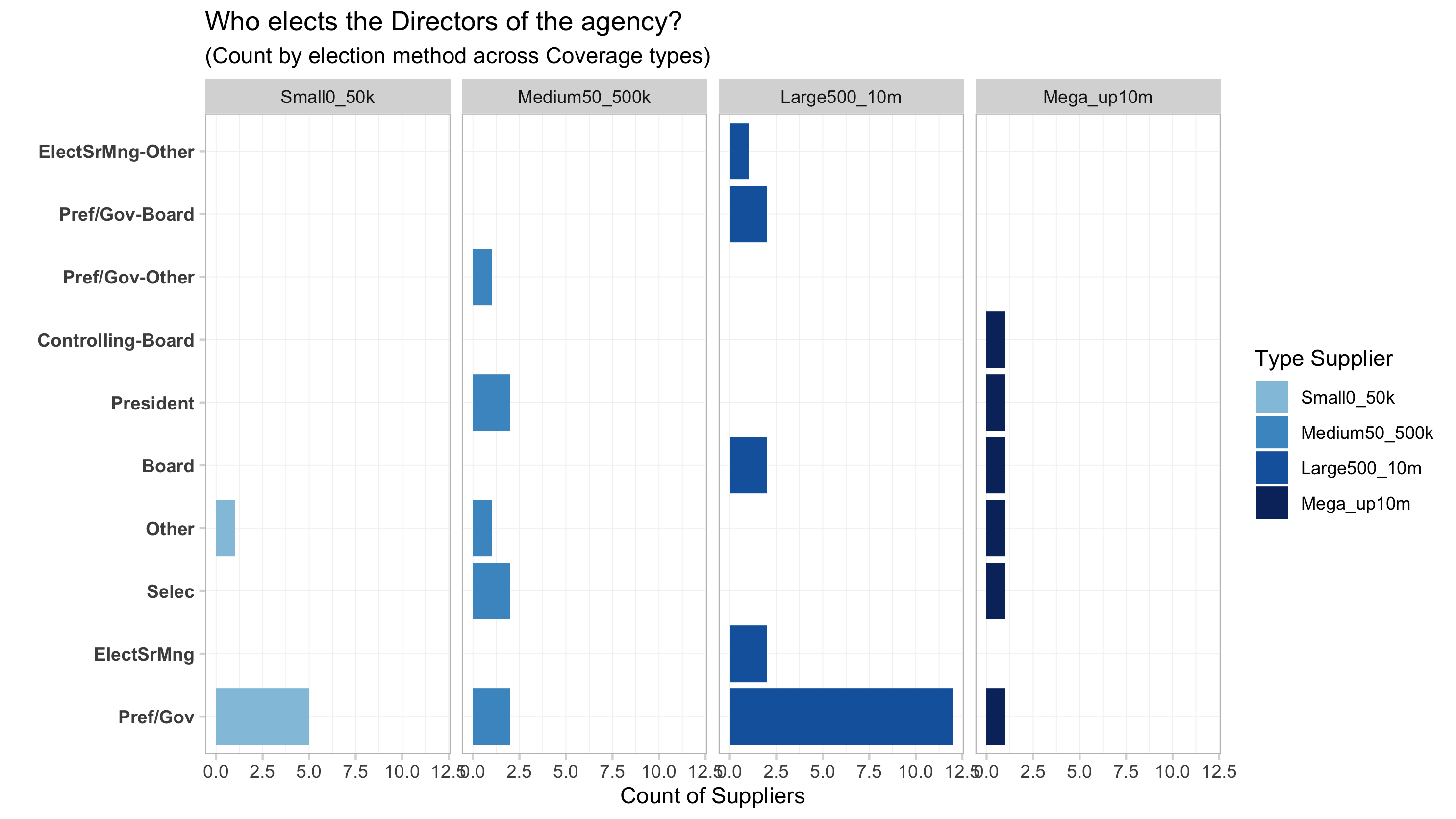
We learned from the survey who is entitled to hire & fire the CEO / President of the agency, his/her remuneration the Sr. Directors.
Appointment of CEO/President/Sr Directors in the Brazil sample
The plots below compare the above across types of ownership and size of the covered area.
- It would appear that the “Prefeito/Gobernador” is in charge in most of the public agencies
- In privately owned suppliers, the Board seems the have the responsability monst cases
4) FINANCIAL HIGHLIGHTS
Lit Input: 1) under-investment + dilapidated infrastructure –> INEFFICIENCIES (see Arniella 2018 ) 2) Energy consumption much of O&M costs (see Lackey and Fillmore 2017)
OPEX by source of financing
Below are the findings from the Brazil sample by group.
load(here::here("output", "tbl_OPEX.Rdata"))
# class(tbl_descstat_cov)

caption <- "Average composition of OPEX - grouped by operator type"

tbl_OPEX_site <-    pandoc.table.return(tbl_OPEX,
                              keep.line.breaks = TRUE,
                              split.tables = Inf,
                              round = 2, big.mark = ",",
                              justify = "lllrrrr",
                              caption = caption,
                              style = "simple",
                              missing = "")  %>%
cat()| Ownership condition | Population coverage size | % OPEX from tariffs (mean) | % OPEX from subsidy (mean) | % OPEX from lending (mean) | % OPEX from other (mean) | N |
|---|---|---|---|---|---|---|
| Public | Small0_50k | 100 | 0 | 0 | 0 | 6 |
| Medium50_500k | 98.33 | 0.83 | 0.83 | 0 | 6 | |
| Large500_10m | 100 | 0 | 0 | 0 | 5 | |
| Mega_up10m | 1 | |||||
| Total | 99.33 | 0.33 | 0.33 | 0 | 18 | |
| Private | Medium50_500k | 100 | 0 | 0 | 0 | 1 |
| Large500_10m | 90 | 0 | 10 | 0 | 3 | |
| Total | 92.5 | 0 | 7.5 | 0 | 4 | |
| Other | Medium50_500k | 100 | 0 | 0 | 0 | 1 |
| Large500_10m | 95.78 | 4.22 | 0 | 0 | 11 | |
| Mega_up10m | 100 | 0 | 0 | 0 | 5 | |
| Total | 97.27 | 2.73 | 0 | 0 | 17 | |
| Total | 97.6 | 1.43 | 0.97 | 0 | 39 |
CAPEX by source of financing
Below are the findings from the Brazil sample by group.
load(here::here("output", "tbl_CAPEX.Rdata"))
# class(tbl_descstat_cov)

caption <- "Average composition of CAPEX - grouped by operator type"

tbl_CAPEX_site <-
    pandoc.table.return(tbl_CAPEX,
    keep.line.breaks = TRUE,
    split.tables = Inf,
    round = 2, big.mark = ",",
    justify = "lllrrrr",
    caption = caption,
    style = "simple",
    missing = "") %>%
cat()| Ownership condition | Population coverage size | % CAPEX from tariffs (mean) | % CAPEX from subsidy (mean) | % CAPEX from lending (mean) | % CAPEX from other (mean) | N |
|---|---|---|---|---|---|---|
| Public | Small0_50k | 100 | 0 | 0 | 0 | 6 |
| Medium50_500k | 92 | 7 | 1 | 0 | 6 | |
| Large500_10m | 50.83 | 37.87 | 11.3 | 0 | 5 | |
| Mega_up10m | 0 | 0 | 100 | 0 | 1 | |
| Total | 73.86 | 13.51 | 12.63 | 0 | 18 | |
| Private | Medium50_500k | 50 | 50 | 0 | 0 | 1 |
| Large500_10m | 40 | 0 | 60 | 0 | 3 | |
| Total | 43.33 | 16.67 | 40 | 0 | 4 | |
| Other | Medium50_500k | 100 | 0 | 0 | 0 | 1 |
| Large500_10m | 34.54 | 40.85 | 10.34 | 15.3 | 11 | |
| Mega_up10m | 34.5 | 10 | 43 | 12.5 | 5 | |
| Total | 39.57 | 32.96 | 14.92 | 13.69 | 17 | |
| Total | 53.96 | 23.23 | 16.84 | 6.59 | 39 |
Foreign participation in capital
Only 6 (out of 39) companies declare they have participation of foreign capital and - of those - the average share is 35%.
5) TARIFFS
IADB (?): we have no idea if tariffs are low or high in LAC (people say are too low, but in fact they are not showing in the Database)
Fixed tariff component
load(here::here("output", "tbl_Fixed_Crit.Rdata"))
# class(tbl_descstat_cov)
caption <- "Determinants of Tariff Fixed Components"
tbl_Fixed_Crit_site <-  pandoc.table.return(tbl_Fixed_Crit,
                                                 keep.line.breaks = TRUE,
                                                 split.tables = Inf,
                                                 round = 2, big.mark = ",",
                                                 justify = "lcrrrr",
                                                 caption = caption,
                                                 style = "simple"#,
                                                 #missing = ""
) %>% cat()| Q14_Tar_Fix_Has | Fixed Component? (N) | Flat | Income/Social | Location type | Consumer type |
|---|---|---|---|---|---|
| Yes | 34 | 14.71% | 79.41% | 17.65% | 88.24% |
| No | 5 | NA% | NA% | NA% | NA% |
Variable tariff component
load(here::here("output", "tbl_Variable_Crit.Rdata"))
# class(tbl_descstat_cov)
caption <- "Determinants of Tariff Variable Components"
tbl_Variable_Crit_site <-   pandoc.table.return(tbl_Variable_Crit,
                                                         keep.line.breaks = TRUE,
                                                         split.tables = Inf,
                                                         round = 2, big.mark = ",",
                                                         justify = "lcrrrrrr",
                                                         caption = caption,
                                                         style = "simple"#,
                                                         #missing = ""
) %>% cat()| Q15_Tar_Var_Has | Variable Component? (N) | Constant Marginal | Increasing Blocks | Decreasing Blocks | Income/Social | Consumer Location | Consumer type |
|---|---|---|---|---|---|---|---|
| Yes | 39 | 2.56% | 94.87% | 5.13% | 92.31% | 7.69% | 94.87% |
Latest 3 changes in tariffs
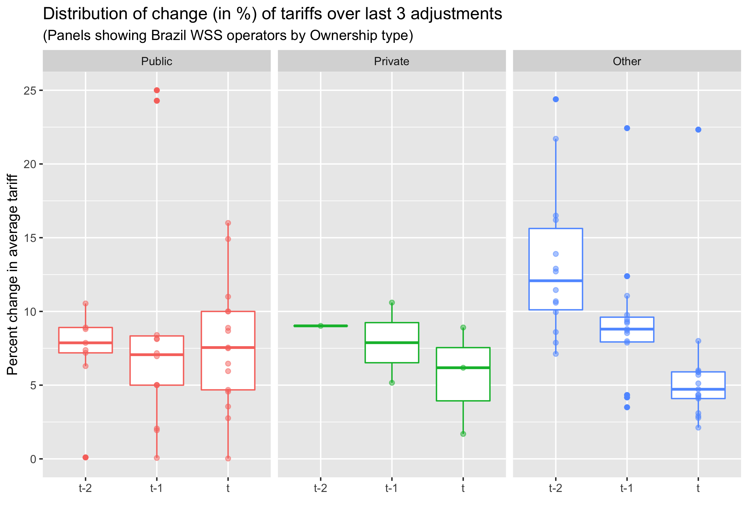
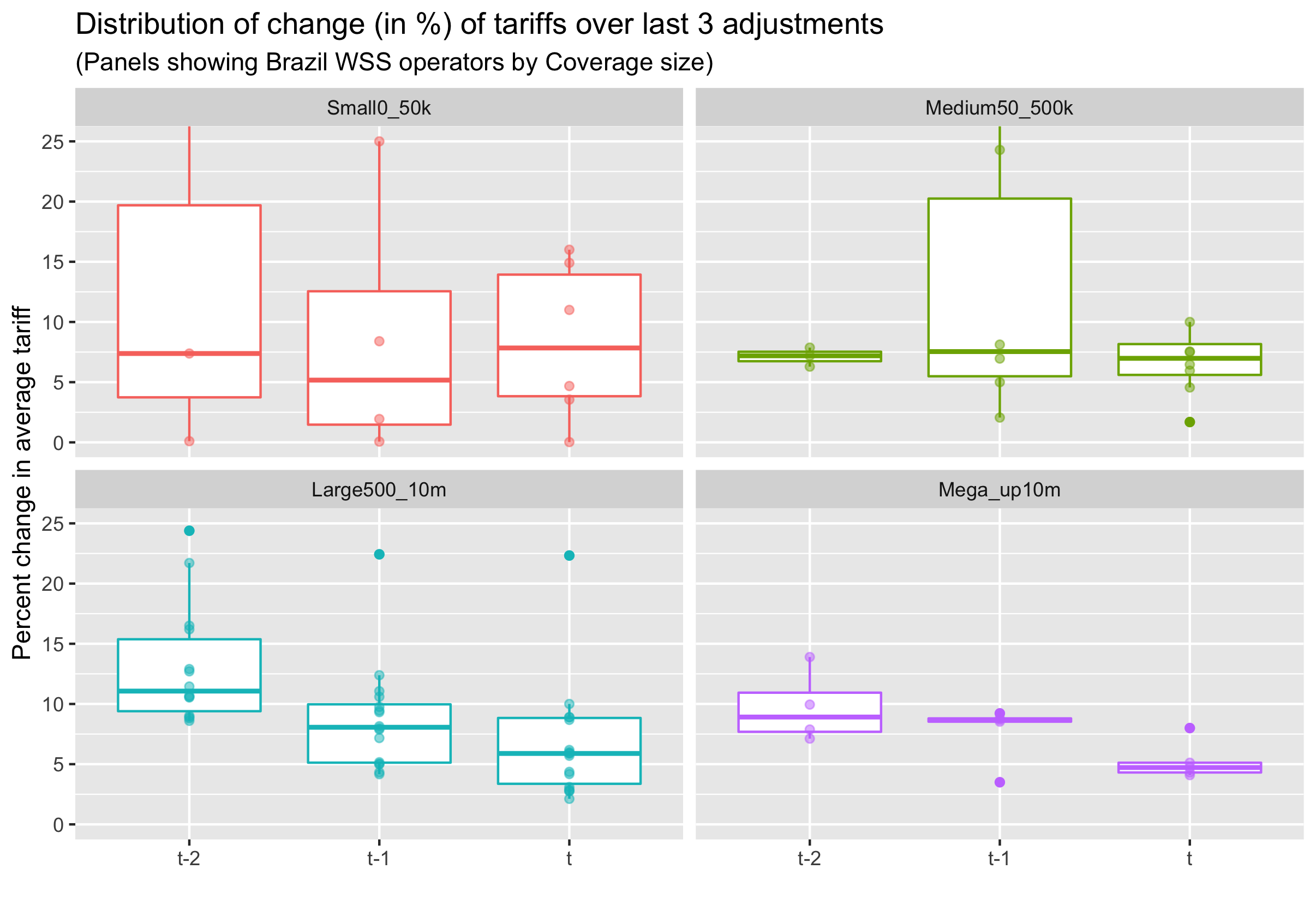
The survey asked the WSS providers the date and % change of the three more recent tariff changes. The plots below show the distribution of the latest adjustment (percentage change to average tariff) across types of ownership and size of the covered area. Depending on the operator:
- “t-2” was some time between 2008 and 2017
- “t-1” was some time between 2007 and 2018
- “t” (or the latest change) was some time between 2014 and 2019
REFERENCE
Later on, I would like to explore if (?) Is the urbanization process (size, local distribution, rate) causing the lack (access, quality, affordability ) to service in the region (controlling for physical assets / hydrological condition, pop #, etc) ? ??↩︎